The effect of tangential velocities

It was first noted by Rezzolla, Zanotti and Pons that there is one effect that is specific to relativistic Riemann problems. Thanks to the Lorentz factor coupling the tangential velocities more tightly to the other terms, it is possible to change the wave pattern in the problem solely by changing the tangential velocity. This cannot happen in the Newtonian case.

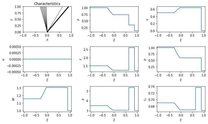
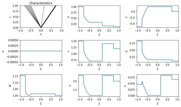
The examples used in their paper use a modified relativistic Sod problem as a base. We set that problem up first:

from r3d2 import eos_defns, State, RiemannProblem
from IPython.display import display, display_png

eos = eos_defns.eos_gamma_law(5.0/3.0)
U_left_sod_modified = State(1.0, 0.5, 0.0, 1.5, eos)
U_right_sod_modified = State(0.125, 0.0, 0.0, 1.2, eos)
rp_sod_modified = RiemannProblem(U_left_sod_modified, U_right_sod_modified)
display(rp_sod_modified)
display_png(rp_sod_modified)

\begin{equation}\begin{cases} \begin{pmatrix} \rho \\ v_x \\ v_t \\ \epsilon \end{pmatrix}= \begin{pmatrix} 1.0000 \\ 0.5000 \\ 0.0000 \\ 1.5000 \end{pmatrix},\\ \begin{pmatrix} \rho \\ v_x \\ v_t \\ \epsilon \end{pmatrix}= \begin{pmatrix} 0.1250 \\ 0.0000 \\ 0.0000 \\ 1.2000 \end{pmatrix}, \end{cases} \quad \implies \quad {\cal R}_{\leftarrow}{\cal C}{\cal S}_{\rightarrow}, \quad p_* = 0.5974, \quad\begin{cases} {\cal R}_{\leftarrow}: \lambda^{(0)}\in [-0.2902, -0.0488],\\ {\cal C}: \lambda^{(1)}= 0.6407,\\ {\cal S}_{\rightarrow}: \lambda^{(2)}= 0.8900, \end{cases} \quad \begin{cases} \begin{pmatrix} \rho \\ v_x \\ v_t \\ \epsilon \end{pmatrix}_{\star_L} = \begin{pmatrix} 0.7341 \\ 0.6407 \\ 0.0000 \\ 1.2207 \end{pmatrix},\\ \begin{pmatrix} \rho \\ v_x \\ v_t \\ \epsilon \end{pmatrix}_{\star_R} = \begin{pmatrix} 0.3427 \\ 0.6407 \\ 0.0000 \\ 2.6154 \end{pmatrix}. \end{cases}\end{equation}

We see the wave pattern has a left going rarefaction and a right going shock.

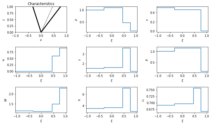
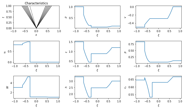
Now, by modifying the tangential velocity of the right state, the wave pattern changes:

U_right_vt_0_9 = State(0.125, 0.0, 0.9, 1.2, eos)
rp_vt_0_9 = RiemannProblem(U_left_sod_modified, U_right_vt_0_9)
display(rp_vt_0_9)
display_png(rp_vt_0_9)

\begin{equation}\begin{cases} \begin{pmatrix} \rho \\ v_x \\ v_t \\ \epsilon \end{pmatrix}= \begin{pmatrix} 1.0000 \\ 0.5000 \\ 0.0000 \\ 1.5000 \end{pmatrix},\\ \begin{pmatrix} \rho \\ v_x \\ v_t \\ \epsilon \end{pmatrix}= \begin{pmatrix} 0.1250 \\ 0.0000 \\ 0.9000 \\ 1.2000 \end{pmatrix}, \end{cases} \quad \implies \quad {\cal S}_{\leftarrow}{\cal C}{\cal S}_{\rightarrow}, \quad p_* = 1.1509, \quad\begin{cases} {\cal S}_{\leftarrow}: \lambda^{(0)}= -0.3224,\\ {\cal C}: \lambda^{(1)}= 0.4549,\\ {\cal S}_{\rightarrow}: \lambda^{(2)}= 0.7638, \end{cases} \quad \begin{cases} \begin{pmatrix} \rho \\ v_x \\ v_t \\ \epsilon \end{pmatrix}_{\star_L} = \begin{pmatrix} 1.0879 \\ 0.4549 \\ 0.0000 \\ 1.5868 \end{pmatrix},\\ \begin{pmatrix} \rho \\ v_x \\ v_t \\ \epsilon \end{pmatrix}_{\star_R} = \begin{pmatrix} 0.4748 \\ 0.4549 \\ 0.5873 \\ 3.6363 \end{pmatrix}. \end{cases}\end{equation}

The result is a left going shock, rather than a rarefaction.

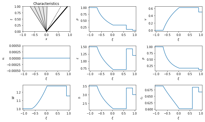
A shock-rarefaction problem can be modified, via a tangential velocity, to a two rarefaction problem in a similar fashion:

U_left_sod_modified2 = State(1.0, 0., 0.0, 1.5, eos)
U_right_sod_modified2 = State(0.125, 0.5, 0.0, 1.2, eos)
rp_sod_modified2 = RiemannProblem(U_left_sod_modified2, U_right_sod_modified2)
display(rp_sod_modified2)
display_png(rp_sod_modified2)

\begin{equation}\begin{cases} \begin{pmatrix} \rho \\ v_x \\ v_t \\ \epsilon \end{pmatrix}= \begin{pmatrix} 1.0000 \\ 0.0000 \\ 0.0000 \\ 1.5000 \end{pmatrix},\\ \begin{pmatrix} \rho \\ v_x \\ v_t \\ \epsilon \end{pmatrix}= \begin{pmatrix} 0.1250 \\ 0.5000 \\ 0.0000 \\ 1.2000 \end{pmatrix}, \end{cases} \quad \implies \quad {\cal R}_{\leftarrow}{\cal C}{\cal S}_{\rightarrow}, \quad p_* = 0.1546, \quad\begin{cases} {\cal R}_{\leftarrow}: \lambda^{(0)}\in [-0.6901, 0.0309],\\ {\cal C}: \lambda^{(1)}= 0.6206,\\ {\cal S}_{\rightarrow}: \lambda^{(2)}= 0.8996, \end{cases} \quad \begin{cases} \begin{pmatrix} \rho \\ v_x \\ v_t \\ \epsilon \end{pmatrix}_{\star_L} = \begin{pmatrix} 0.3262 \\ 0.6206 \\ 0.0000 \\ 0.7108 \end{pmatrix},\\ \begin{pmatrix} \rho \\ v_x \\ v_t \\ \epsilon \end{pmatrix}_{\star_R} = \begin{pmatrix} 0.1621 \\ 0.6206 \\ 0.0000 \\ 1.4302 \end{pmatrix}. \end{cases}\end{equation}

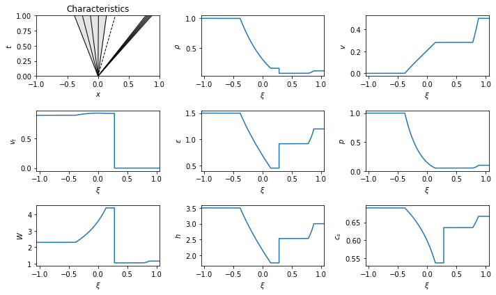
And now with tangential velocity:

U_left_vt_0_9 = State(1.0, 0.0, 0.9, 1.5, eos)
rp2_vt_0_9 = RiemannProblem(U_left_vt_0_9, U_right_sod_modified2)
display(rp2_vt_0_9)
display_png(rp2_vt_0_9)

\begin{equation}\begin{cases} \begin{pmatrix} \rho \\ v_x \\ v_t \\ \epsilon \end{pmatrix}= \begin{pmatrix} 1.0000 \\ 0.0000 \\ 0.9000 \\ 1.5000 \end{pmatrix},\\ \begin{pmatrix} \rho \\ v_x \\ v_t \\ \epsilon \end{pmatrix}= \begin{pmatrix} 0.1250 \\ 0.5000 \\ 0.0000 \\ 1.2000 \end{pmatrix}, \end{cases} \quad \implies \quad {\cal R}_{\leftarrow}{\cal C}{\cal R}_{\rightarrow}, \quad p_* = 0.0513, \quad\begin{cases} {\cal R}_{\leftarrow}: \lambda^{(0)}\in [-0.3838, 0.1375],\\ {\cal C}: \lambda^{(1)}= 0.2809,\\ {\cal R}_{\rightarrow}: \lambda^{(2)}\in [0.7773, 0.8750], \end{cases} \quad \begin{cases} \begin{pmatrix} \rho \\ v_x \\ v_t \\ \epsilon \end{pmatrix}_{\star_L} = \begin{pmatrix} 0.1683 \\ 0.2809 \\ 0.9324 \\ 0.4573 \end{pmatrix},\\ \begin{pmatrix} \rho \\ v_x \\ v_t \\ \epsilon \end{pmatrix}_{\star_R} = \begin{pmatrix} 0.0838 \\ 0.2809 \\ 0.0000 \\ 0.9189 \end{pmatrix}. \end{cases}\end{equation}

Reactive case

An interesting question is on the potential impact of this relativistic effect on detonations and deflagrations. Let us set up a reference reactive problem and add tangential velocities:

eos_reactive = eos_defns.eos_gamma_law_react(5.0/3.0, 0.25, 1.0, 1.0, eos)
U_reactive = State(1.0, -0.5, 0.0, 1.5, eos_reactive)
U_burnt = State(0.125, 0.0, 0., 1.2, eos)
rp_reactive_base = RiemannProblem(U_reactive, U_burnt)
display(rp_reactive_base)
display_png(rp_reactive_base)

\begin{equation}\begin{cases} \begin{pmatrix} \rho \\ v_x \\ v_t \\ \epsilon \\ q \end{pmatrix}= \begin{pmatrix} 1.0000 \\ -0.5000 \\ 0.0000 \\ 1.5000 \\ 0.2500 \end{pmatrix},\\ \begin{pmatrix} \rho \\ v_x \\ v_t \\ \epsilon \end{pmatrix}= \begin{pmatrix} 0.1250 \\ 0.0000 \\ 0.0000 \\ 1.2000 \end{pmatrix}, \end{cases} \quad \implies \quad \left({\cal CJDF}_{\leftarrow}{\cal R}_{\leftarrow}\right) {\cal C}{\cal S}_{\rightarrow}, \quad p_* = 0.1464, \quad\begin{cases} \left({\cal CJDF}_{\leftarrow}{\cal R}_{\leftarrow}\right) : \lambda^{(0)}\in [-0.7887, -0.4919],\\ {\cal C}: \lambda^{(1)}= 0.1532,\\ {\cal S}_{\rightarrow}: \lambda^{(2)}= 0.7187, \end{cases} \quad \begin{cases} \begin{pmatrix} \rho \\ v_x \\ v_t \\ \epsilon \end{pmatrix}_{\star_L} = \begin{pmatrix} 0.3120 \\ 0.1532 \\ 0.0000 \\ 0.7039 \end{pmatrix},\\ \begin{pmatrix} \rho \\ v_x \\ v_t \\ \epsilon \end{pmatrix}_{\star_R} = \begin{pmatrix} 0.1570 \\ 0.1532 \\ 0.0000 \\ 1.3989 \end{pmatrix}. \end{cases}\end{equation}

We see that this is a deflagration-shock problem.

Now add tangential velocities to the unburnt material:

U_reactive_vt_0_9 = State(1.0, -0.5, 0.8, 1.5, eos_reactive)
rp_reactive_vt_reactive = RiemannProblem(U_reactive_vt_0_9, U_burnt)
display(rp_reactive_vt_reactive)
display_png(rp_reactive_vt_reactive)

\begin{equation}\begin{cases} \begin{pmatrix} \rho \\ v_x \\ v_t \\ \epsilon \\ q \end{pmatrix}= \begin{pmatrix} 1.0000 \\ -0.5000 \\ 0.8000 \\ 1.5000 \\ 0.2500 \end{pmatrix},\\ \begin{pmatrix} \rho \\ v_x \\ v_t \\ \epsilon \end{pmatrix}= \begin{pmatrix} 0.1250 \\ 0.0000 \\ 0.0000 \\ 1.2000 \end{pmatrix}, \end{cases} \quad \implies \quad \left({\cal CJDF}_{\leftarrow}{\cal R}_{\leftarrow}\right) {\cal C}{\cal R}_{\rightarrow}, \quad p_* = 0.0464, \quad\begin{cases} \left({\cal CJDF}_{\leftarrow}{\cal R}_{\leftarrow}\right) : \lambda^{(0)}\in [-0.6382, -0.4005],\\ {\cal C}: \lambda^{(1)}= -0.2901,\\ {\cal R}_{\rightarrow}: \lambda^{(2)}\in [0.4159, 0.6667], \end{cases} \quad \begin{cases} \begin{pmatrix} \rho \\ v_x \\ v_t \\ \epsilon \end{pmatrix}_{\star_L} = \begin{pmatrix} 0.1567 \\ -0.2901 \\ 0.9377 \\ 0.4445 \end{pmatrix},\\ \begin{pmatrix} \rho \\ v_x \\ v_t \\ \epsilon \end{pmatrix}_{\star_R} = \begin{pmatrix} 0.0789 \\ -0.2901 \\ 0.0000 \\ 0.8828 \end{pmatrix}. \end{cases}\end{equation}

Again, by adding tangential velocities to the right state the shock has become a rarefaction.